ABSTRACT. Up to now, MegaCam exposure time calculator assumes a model of aperture photometry, and computes required exposure times to obtain a given SNR in the “optimal” aperture for a given set of background, instrumental source magnitude, seeing, and read-out noise. Optimality is here defined with respect to the aperture radius that maximises the SNR keeping everything else fixed.
With the development of PSF photometry in recent versions of SExtractor, it becomes interesting to revisit the exposure time calculations to obtain a given SNR on a source flux measured by fitting a PSF shape on the source by adjusting both the amplitude (flux) of the source and its position.
In this document, we will describe a traditional Fisher matrix approach to the problem, that gives a robust lower limit on the SNR of such a measurement for a given exposure time (and background, source magnitude, etc.), or conversely a lower limit on the exposure time required to achieve a given SNR on such a parametric (maximum likelihood) measurement of the source flux.
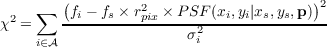
Let us assume that the measurement error on the value of the flux of the source in a given pixel is gaussian distributed (a reasonable assumption as long as the sum of the background and source counts is large enough). The PSF photometry then proceeds by minimizing the following χ2:
where fi is the measured flux in pixel i (in ADU), fs is the (integrated,
total) source flux (in ADU), and rpix2 × PSF(xi,yi|xs,ys,p) is the
(adimensional) Point Spread Function (approximately) integrated in pixel i
1(located
at position xi,yi) with a source position xs,ys, and other additional parameters p, and
 is a (large) aperture centered on the source position. This χ2is minimized jointly with
respect to the source parameters (xs,ys,fs) and eventually (a subset of) the PSF-specific
parameters p.
is a (large) aperture centered on the source position. This χ2is minimized jointly with
respect to the source parameters (xs,ys,fs) and eventually (a subset of) the PSF-specific
parameters p.
In the following, we will assume that the PSF is a normalized Moffat function whose parameters (α = hwhm and β) are perfectly known (limiting case of a PSF extraction from a large number of stellar sources). In practice, there should be some correlation of errors between the PSF shape reconstruction and the flux measurements of sources that were used to reconstruct the PSF shape, but we will ignore them in the following calculations.
We will thus consider the errors on the estimates of the parameters of a single source
 s,
s, s,
s, s, using the Fisher matrix formalism. This will give us robust lower limits on the
required integration time needed to achieve a given SNR on the source flux. We will
consider three independent sources of noise: read-out noise, background photon noise and
source photon noise.
s, using the Fisher matrix formalism. This will give us robust lower limits on the
required integration time needed to achieve a given SNR on the source flux. We will
consider three independent sources of noise: read-out noise, background photon noise and
source photon noise.
Let us recall the shape of the normalized Moffat profile:
![[ ]- β
M (xi,yi|xs,ys,α,β) = (β --1)(21∕β-- 1) 1+ (21∕β - 1)(xi --xs)2 +-(yi --ys)2
π α2 α2](PSF-photometry4x.png) | (1.1) |
M is normalized such that ∫ dxidyiM(xi,yi|xs,ys,α,β) = 1. Its derivative with respect to the source position (xs or ys), which we will need later on, is given by:
![1∕β [ 2 2]-(β+1)
∂M--= 2β(β---1)(24-----1)×(xi- xs)× 1 + (21∕β - 1)(xi --xs)-+2(yi --ys)
∂xs πα α](PSF-photometry5x.png)
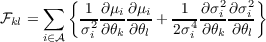
With the assumption of Gaussian errors, the Fisher matrix takes a simple form:
where P is the (joint) probability distribution of all pixel measurements in the aperture, θ is the array of the source parameters (here xs,ys,fs), and μand Σ are respectively
the mean vector and covariance matrix of the pixel flux measurements. If we make the
(traditional) assumption of uncorrelated pixel noise, then the matrix Σ becomes
diagonal, with entries per pixel:
 | (2.2) |
where b is the integrated sky background value per pixel in ADU (assumed constant over the aperture), g is the gain in e-∕ADU (also assumed constant over the aperture), Nccd is the readout noise variance in ADU2(also assumed constant over the aperture). The mean value of the (sky-subtracted) pixel flux simply reads
 | (2.3) |
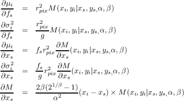
We thus only need to compute the first derivatives of the Equations 2.2,2.3 w.r.t. the source parameters, to obtain the expression of the correponding Fisher matrix elements. Using the expression of the Moffat profile from Equation 1.1, we have:
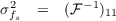
Taking the source parameters to be (fs,xs,ys) in that order, then (a lower limit on) the variance of the flux estimate, marginalized over source position, is given by:

where trans is the atmospheric transmission, ZADU = Ze-- 2.5log 10(g) is the zeropoint in ADUs, k is the airmass-dependent extinction coefficient, and am is the airmass.
Note that for a centrally symmetric PSF there is no correlation of errors between the
position parameters xs,ys of the source and the source flux fs, hence in this case we
have  12 = 13 = 0, and σfs2 = 1∕11. Also, if the PSF is azimuthally symmetric, then
there is no correlation of error between xs and ys (hence the Fisher matrix is diagonal in
this case).
12 = 13 = 0, and σfs2 = 1∕11. Also, if the PSF is azimuthally symmetric, then
there is no correlation of error between xs and ys (hence the Fisher matrix is diagonal in
this case).
The derivation given above gives an exposure time for a given SNR. The reverse function (DIET) cannot be written easily explicitely, but can be numerically computed using a simple root finding algorithm.
![2
Fkl = - ⟨∂-lnP-⟩
∂θk∂θl [ ]
∂μT- -1∂μ- 1 -1 ∂Σ - 1∂Σ-
(2.1) = ∂θk Σ ∂θl + 2tr Σ ∂θkΣ ∂θl](PSF-photometry6x.png)