1. Formulation of the problem

The photometric equation allows us to relate the AB (instrumental) magnitude mAB of a given star to the total flux (in e^-∕s):

(1.1)

the total flux for a given exposure time t_exp being simply given by F_tot = F_et_exp. In equation 1.1, transis the atmospheric transmission at zenith at the time of the exposure, ZP is the zero point in e^-∕s in the given band, am is the airmass of the exposure, and k is an airmass-dependent slope of the atmospheric extinction. To compute the signal to noise in an aperture, we will also need the total background flux in e^-∕s∕pixel

(1.2)

Finally, the Point Spread Function of the CFHT imagers are well represented by a Moffat function:

(1.3)

where R is the angular distance (radius) from the point source in arcsec, α = IQ∕2 (where IQ, the Image Quality or “seeing”, is defined as the full width at half maximum of the PSF), and β = 3 is a good fit to both MegaCam and WirCam. The flux fraction contained within an aperture of radius R is thus:

(1.4)

This allows us to write the expression of the signal-to-noise for the flux measured in a circular aperture of radius R:

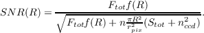(1.5)

The noise contributions in the numerator include the photon noise variance from both the source and the background, and the readout-noise variance n_ccd². These last two quantities are expressed per pixel area, hence the π(R∕r_pix)²factor. Finally, n_C is a fudge factor that can account for possible spatial correlations in the noise, it will be set to n_C = 1 (no correlation) in the ETC.

2. Computing SNR at optimal radius (and others)

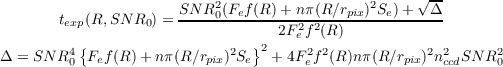
For a fixed exposure time, equation 1.5 gives the expression of the signal-to-noise in the aperture as a function of the aperture radius. We seek to find R_opt the optimal radius that maximizes this quantity. Starting from equation 1.5, and defining F(R) = F_totf(R), we get:

(2.1)

which is solved by a simple root finder. Equation 1.5 is then used to compute the corresponding the optimal signal-to-noise ratio.

Of course, the same equation can be used to compute the SNR in any given aperture. For instance, the “large aperture” mode of the ETC corresponds to the case where

(2.2)

This aperture, for a Moffat profile (equation 1.3) with β = 3, includes ~ 96.24% of the total flux of the source.

3. Computing exposure time at optimal radius (and others)

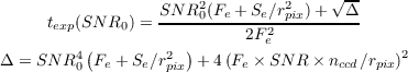
Starting from equation 1.5, and recalling that F_tot = F_e ×t_exp, we can solve for t_exp at fixed SNR = SNR₀. Indeed it is the solution of a second degree polynomial equation:

(3.1)

4. Case of extended sources

This case turns out to be a simpler version of the formulation above. The photometric equation 1.1 can be used as written, but the fluxes (as well as the magnitudes) are to be understood per 1arcsec² aperture. In such an aperture, the total flux is then simply given by F_e × t_exp. Equation 1.5 then reads:

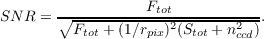
Solving for t_expat fixed SNR, we get:

(4.1)

5. Case of galaxies with Sérsic profiles

In the case of extended objects like galaxies, which are still characterized with a total magnitude like point sources, but also exhibit an intensity profile I(r) that is not negligible in size compared to the PSF extent, a specific treatment is necessary. Indeed, in this case, Eq. 1.5 is still valid, but Eq. 1.4, which is valid for a point source, needs to be modified to account for the extension of the galaxy. Let us model the galaxy intensity profiles as general Sérsic profiles:

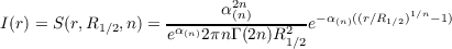(5.1)

with R_1∕2the half-light radius of the intensity profile, n the profile index, and α_(n) is a normalization constant such that Γ(2n) = 2γ(2n,α_(n)) where γ(n,x) is the incomplete Gamma function of index n. The intensity profile of Eq. 5.1 is impacted by the seeing, so that the observed intensity profile is the convolution of the profile of Eq. 5.1 with the Moffat profile of the PSF given by Eq. 1.3. There is unfortunately no simple close form for this convolution [Trujillo et al., 2001].

However, both Sérsic and Moffat profiles can be adequately approximated by mixtures of gaussian profiles, which again produce mixtures of gaussian profiles after convolving one by the other. Also, mixture of gaussian profiles can be easily scaled, as to match the PSF seeing and galaxy half-light radius, so that the approximations, parametrized by the weights and variances of the mixture of gaussians, can be precomputed once for all.

In practice, these parameters are computed for integer values of the Sérsic index n ∈{1,...,5}, and a Moffat parameter β = 3 which is a good match for the PSF of both imaging CFHT instruments. The computation has been done using the relevant part of The Tractor software http://thetractor.org, as described in Hogg and Lang [2013]. Following the latter, let us define a mixture of gaussian profiles in the following way:

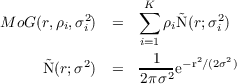
where (r;σ²) is a circularly symmetric, two-dimensional, normalised Gaussian profile, i.e. such that ∫ ₀^∞2πrÑ(r;σ²)dr = 1. This normalisation implies automatically that

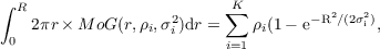
and in particular that ∫ ₀^∞2πr × MoG(r,ρ_i,σ_i²)dr = ∑ _i=1^Kρ_i. The mixtures of Gaussian are thus very easy to normalize. The flux fraction within an aperture of radius R is thus simply given by:

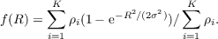(5.2)

To be complete, let us now express the convolution of two mixtures of gaussian profiles. Again, following Hogg and Lang [2013], it is given by the following mixture of gaussian profiles:

which is easily computed. Plugging Eq. 5.2 into the expression of the SNR given by Eq. 1.5, one can then proceed as in Sec. 2 and Sec. 3.

References